From Data Deluge to Clarity: Taming Student Lists with Google Sheets

Have you ever found yourself hunched over a spreadsheet, staring at a sea of student data, desperately needing to pull out specific individuals? It’s a common scenario in education, isn’t it? Whether you’re trying to identify students for an intervention, a special program, or just to send out a targeted communication, the manual scroll-and-select method can feel like trying to find a needle in a digital haystack. While Google Sheets offers a treasure trove of functions, sometimes the most powerful tools aren’t always the prettiest, especially when you’re trying to achieve a specific kind of precision.

The Query Conundrum: Powerful, Yet Peculiar

Ah, the QUERY function. It’s a powerhouse, a bit like having a mini-database language right inside your spreadsheet. For many tasks, it feels like a superpower. But when it comes to filtering a range of data based on a *list* of specific values—like a handful of student IDs—it can get… well, clunky. Trying to construct a beautiful QUERY statement to say “give me all students whose ID is P2 OR P3 OR P4 OR P5 OR P6” quickly turns into a verbose, unwieldy mess that’s difficult to read and even harder to maintain. It’s certainly not pretty, and frankly, it makes you want to face-plant into your keyboard.

Unleashing the Dynamic Duo: FILTER and COUNTIF

Fear not, my fellow educators! There’s a far more elegant and efficient way to achieve this specific filtering magic in Google Sheets: the dynamic duo of FILTER and COUNTIF. This combination is the ultimate “low floor, high ceiling” solution for this particular problem, allowing you to quickly isolate exactly the students you need, or even those you *don’t* need, in a snap. It’s truly about Resolving Everyday data dilemmas with a few lines of logic.

How It Works: A Simple, Speed-Demon Approach

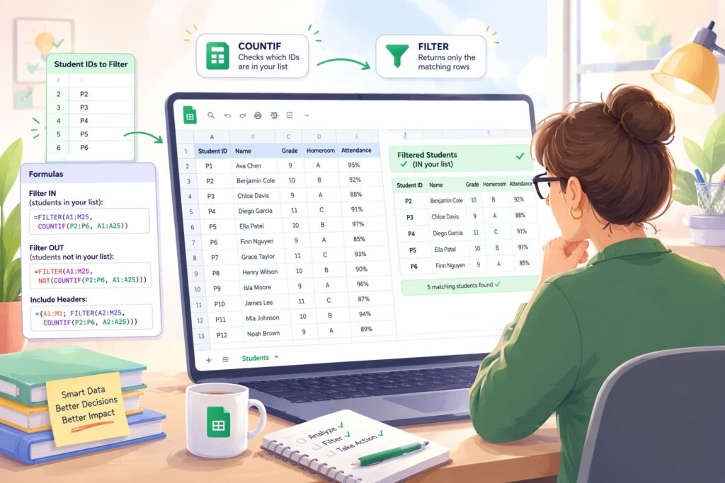
Let’s imagine you have your main student data in a range like A1:M25, with student IDs residing in column A. Then, you have a specific list of student IDs you want to filter for, perhaps in P2:P6. Here’s how you can make this magic happen:

• The Core Formula for Filtering IN:
  =FILTER(A1:M25, COUNTIF(P2:P6, A1:A25))
  What’s happening here? COUNTIF(P2:P6, A1:A25) creates an array of 0s and 1s. For every student ID in A1:A25, if it appears in your list (P2:P6), COUNTIF returns a 1 (or more, if it’s duplicated, but 1 is all FILTER needs). If it doesn’t appear, it returns 0. The FILTER function then simply includes rows where the corresponding COUNTIF result is greater than 0. It’s lightning-fast and incredibly intuitive!
• Filtering OUT (Finding Students NOT in Your List):
  Want to find all students not on your specific list? A tiny tweak makes this possible:
  =FILTER(A1:M25, NOT(COUNTIF(P2:P6, A1:A25)))
  The NOT() function simply inverts the logic, giving you everyone *else*.
• Grabbing That Header Row: The Array Literal Trick
  A common hang-up is how to include your header row consistently with your filtered data. This is where an array literal comes to the rescue! If your header is in row 1, and your data starts from row 2, you can do this:
  ={A1:M1; FILTER(A2:M25, COUNTIF(P2:P6, A2:A25))}
  This concatenates your header row with your filtered data, giving you a complete, clean output. It’s a small but mighty trick that streamlines your reports.

Your Turn to Master the Data Puzzle

I love the algorithmic nature of programming and problem-solving, and this specific Sheets technique is a perfect example of how thinking through a problem with logic can lead to elegant solutions. It’s a puzzle that demands you sharpen your problem-solving skills every single day. This isn’t just about filtering data; it’s about getting better at deconstructing complex problems and becoming more resilient when things don’t work the first time.

Now it’s your turn to make a difference: go out there and light up a mind!

I truly believe that the right systems allow us to focus back on the students rather than the spreadsheets. To help you put this into practice immediately, I’ve built a Filter/COUNTIF Automation Tool that handles the heavy lifting for you.

You can grab this template for free below. I’ll send a PDF guide and your personal ‘Force Copy’ link directly to your inbox so you can get started in seconds.